Core Optimization Algorithms

This section introduces the main scheduling algorithms.

---

Function schedule

Syntax and Algorithm Description

schedule executes the scheduling optimization. Specifically, it selects and runs one of four optimization algorithms depending on the input arguments.

When we run out = schedule(scenario,algorithm_type), it selects to run:

• centralized algorithm for load flattening problem if

  scenario.Problem_type == "Lf" and algorithm_type == "cent"

• distributed algorithm for load flattening problem if

  scenario.Problem_type == "Lf" and algorithm_type == "dist"

• centralized algorithm for user-friendly problem if

  scenario.Problem_type == "Uf" and algorithm_type == "cent"

• distributed algorithm for user-friendly problem if

  scenario.Problem_type == "Uf" and algorithm_type == "dist"

Both centralized and distributed algorithms for load flattening problem are implemented in load_flattening. The distributed algorithm for load flattening problem implemented in load_flattening is developed based on [1] and [2].

Meanwhile, both centralized and distributed algorithms for user-friendly problem are implemented in user_friendly. The distributed algorithm for user-friendly problem implemented in user_friendly is developed based on [3].

For more details about schedule, particularly regarding optional inputs, see schedule. For more details about code implementation of load_flattening or user_friendly, visit GitHub repository.

Output Format

After running schedule, the user gets a structure containing the following fields as an output.

Field	Type	Description
u	T×N_c matrix	Schedule for each charger
cost	scalar	Total cost
scenario	Scenario	Scenario instance
metadata	struct	Metadata about when and how output was generated

If scenario.Problem_type == "Lf", then the output structure also contains a field lam(T×1 matrix), which is a Lagrange multiplier for balance constraint.

Example

We revisit the example from Quick Demo. Data is provided in tutorial/Samples/.

% Preprocess input scenario
jsonfile = "Sample_Lf.json";
scenario = import_scenario(jsonfile);

% Run schedule()
out = schedule(scenario,"cent");

% Inspect the variable
openvar('out')

% Compare schedule u_1 of charger 1
T = out.scenario.T;
U = out.u;

stem(1:T, U(:,1))

Function schedule_rh

Syntax and Algorithm Description

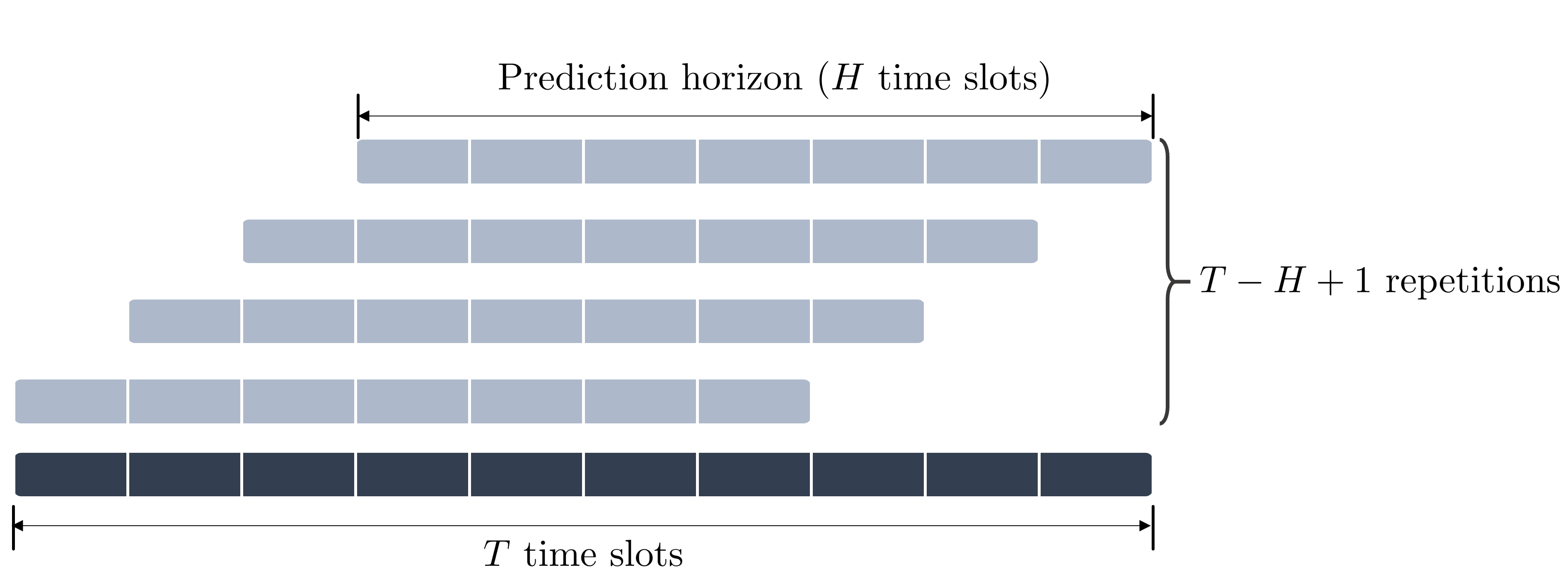
In the real-time scheduling problem, information about future EVs, such as their arrival time slot, departure time slot, initial stored energy, and reference stored energy, is unknown prior to their arrival. In this regard, schedule_rh performs real-time scheduling by repeatedly calling schedule based on the receding horizon scheme.

When out = schedule_rh(scenario,algorithm_type) is executed, the following procedure takes place.

• schedule is called considering only time slots 1, \(\dots\) , H and the EVs connected at time slot 1.

• Here, H is referred to as the length of the prediction horizon.

• Once the scheduling is completed, the charging schedules corresponding to time slot 1 are applied.

• The procedure is then repeated as the prediction horizon recedes by on time slot; that is, schedule is called considering time slots 2, \(\dots\) , H+1 and EVs connected at time slot 2, and so on.

• The algorithm terminates when the prediction horizon can no longer recede, i.e., after scenario.T - H + 1 repetitions of schedule.

• algorithm_type is applied for each execution of schedule.

Output Format

After running schedule_rh, the user gets a structure containing the following fields as an output.

Field	Type	Description
u	(T-H+1)×N_c matrix	Schedule for each charger
cost	scalar	Total cost
scenario	Scenario	Scenario instance of length (T-H+1)
metadata	struct	Metadata about when and how output was generated

If scenario.Problem_type == "Lf", then the output structure also contains a field lam ((T-H+1)×1 matrix), which is a Lagrange multiplier for balance constraint.

Example

We now apply the real-time scheduling algorithm for our example scenario.

% Preprocess input scenario
jsonfile = "Sample_Lf.json";
scenario = import_scenario(jsonfile);

% Run schedule()
H = 12;   % the length of the prediction horizon
out = schedule_rh(scenario,"cent",H=H);

% Inspect the variable
openvar('out')

% Compare schedule u_1 of charger 1
T_rh = out.scenario.T;   % = scenario.T-H+1
U_rh = out.u;

stem(1:T_rh, U_rh(:,1))

---

[1]

J. Heo, S. Hyeon, H. Shim, and J. Kim, “Fully distributed EV charging scheduling for load flattening in V2G sytems,” in Proc. IEEE Conf. Decision Control, 2024.

[2]

J. Heo, J. G. Lee, and H. Shim, “Initialization-free distributed PI algorithm for constraint-coupled optimization,” to be submitted.

[3]

S. Lee, J. Heo, S. Hyeon, J. Nam, H. Shim, and J. Kim, “User-friendly vehicle-to-grid optimal scheduling problem and distributed implementation for plug-and-play operation,” in Proc. Int. Conf. Control Automat. Syst., 2023.