Simulation and Analysis

Here, we introduce application-level simulation tools which help users run automated multi-algorithm and multi-scenario evaluations.

---

simulate() Function

simulate() enables users to run multiple algorithms sequentially under the same scenario, for comparing different algorithms. Specifically, sim_out = schedule(scenario,Name=Value) to use following three types of algorithms:

• oracle: if input argument oracle = true(default) is given, it performs oracle scheduling which means scheduling with full future knowledge

• cent: if input argument cent = true is given, it performs centralized receding horizon scheduling

• dist: if input argument dist = true is given, it performs distributed receding horizon scheduling

For more details about simulate(), particularly regarding optional inputs, see simulate.

Output Format

After running simulate(), the user gets a structure containing the following fields as an output.

Field	Type	Description
oracle	logical	Performed oracle scheduling or not
cent	logical	Performed centralized receding horizon scheduling or not
dist	logical	Performed distributed receding horizon scheduling or not
Problem_type	“Lf”|”Uf”	Type of problem, either “Lf” for load flattening or “Uf” for user-friendly
monte_carlo	always false	Whether it is Monte-Carlo Simulation or not
N_sim	always 1	Number of scenarios
results	struct	Structure containing common scenario and oracle/cent/dist scheduling results

sim_out.monte_carlo is a flag that indicates whether sim_out is the output of the simulate() function or of the simulate_mc() function.

Example

The following example shows how to run simulate() for the example scenario.

% Set parameters
T0 = 24;
H = 6;
N_c = 20;
L = -ones(N_c+1);
for i=1:N_c+1
    L(i,i) = N_c;
end
arrival_rates = [1*ones(8,1); 3*ones(8,1); 1*ones(8,1); 3*ones(5,1)];
mean_stay_duration = 3*60;

% Create a scenario generator
gen = PoissonScenarioGenerator("Problem_type","Lf",'T',T0+H-1,...
    'N_c',N_c,'L',L,'arrival_rates',arrival_rates,...
    'mean_stay_duration',mean_stay_duration);

% Run simulate() for oracle and cent algorithm
sc = generate(gen);
sim_out = simulate(sc,H=H,cent=true);

% Save the data
save("sim_out_Lf.mat","-struct","sim_out");

simulate_mc() Function

simulate_mc() repeats simulate() several times in order to perform Monte-Carlo evaluation.

When we run mc_out = schedule(gen,N_sim,Name=Value) for PoissonScenarioGenerator object gen, it repeatedly generate scenario using same scenario generator gen, N_sim times. For each scenario, it calls simulate().

For more details about simulate_mc(), particularly regarding optional inputs, see simulate.

Tip

You can use any MyOwnScenarioGenerator inheriting AbstractScenarioGenerator as an input of simulate_mc()

Output Format

After running simulate_mc(), the user gets a structure containing the following fields as an output.

Field	Type	Description
oracle	logical	Performed oracle scheduling or not
cent	logical	Performed centralized receding horizon scheduling or not
dist	logical	Performed distributed receding horizon scheduling or not
Problem_type	“Lf”|”Uf”	Type of problem, either “Lf” for load flattening or “Uf” for user-friendly
monte_carlo	always true	Whether it is Monte-Carlo Simulation or not
N_sim	positive integer	Number of scenarios
results	N_sim×1 struct array	Structure containing common scenario and oracle/cent/dist scheduling results

Since scenarios in repeated simulations are generated from the same scenario generator gen, they share the same properties such as Problem_type,N_c,T,Delta,etc.

Example

The following example shows how to run simulate_mc() for the example scenario.

% Set parameters
N_sim = 3;
T0 = 24;
H = 6;
N_c = 20;
L = -ones(N_c+1);
for i=1:N_c+1
    L(i,i) = N_c;
end
arrival_rates = [1*ones(8,1); 3*ones(8,1); 1*ones(8,1); 3*ones(5,1)];
mean_stay_duration = 3*60;

% Create a scenario generator
gen = PoissonScenarioGenerator("Problem_type","Lf",'T',T0+H-1,...
    'N_c',N_c,'L',L,'arrival_rates',arrival_rates,...
    'mean_stay_duration',mean_stay_duration);

% Run simulate_mc() for oracle and cent algorithm
mc_out = simulate_mc(gen,N_sim,H=H,cent=true);

% Save the data
save("mc_out_Lf.mat","-struct","mc_out");

analyze() Function

As well as automated functions of running multiple algorithms, we provide a visualization and analysis tool for users.

analyze() is created using matlab app designer, various performance metrics are given by interactive plots. Users can compare oracle, centralized-RH, and distributed-RH scheduling methods under identical simulation settings.

Following four examples show what can analyze() do. For more details about analyze(), such as loading data directly from a Workspace, see analyze.

Analyze Single-Scenario Result (Load Flattening)

In this example, the output of simulate() function for a load flattening scenario is required. It can be generated manually following the earlier example, or obtained from the sim_out_Lf.mat located in the tutorial/Samples/ folder.

% Load output
sim_out = load("sim_out_Lf.mat");

% analyze()
analyze(data=sim_out);

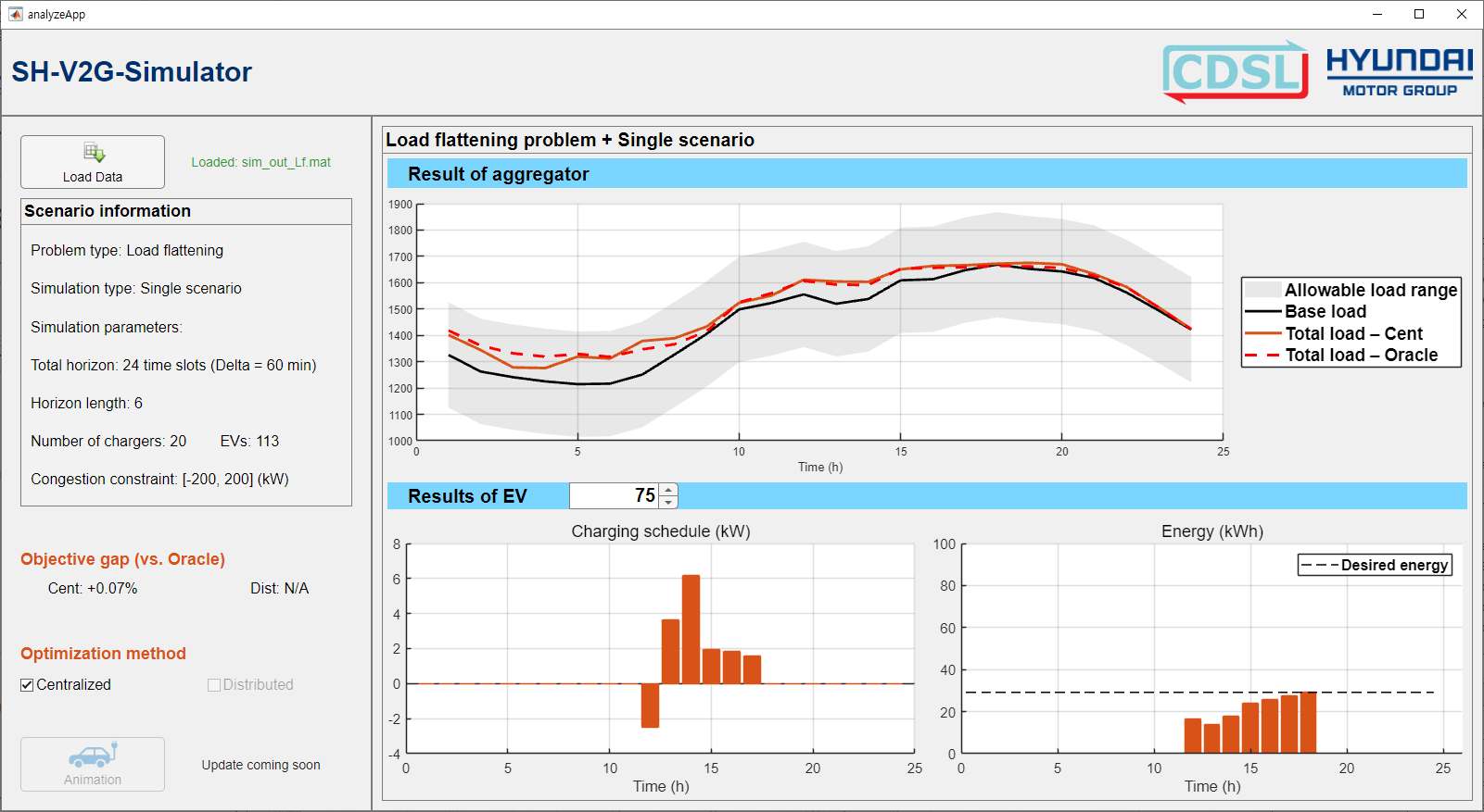
analyze helps evaluating the grid-level performance.

Analyze Single-Scenario Result (User-Friendly)

In this example, the output of simulate() function for a user-friendly scenario is required. It can be generated manually following the earlier example, or obtained from the sim_out_Uf.mat located in the tutorial/Samples folder.

% Load output
sim_out = load("sim_out_Uf.mat");

% analyze()
analyze(data=sim_out);

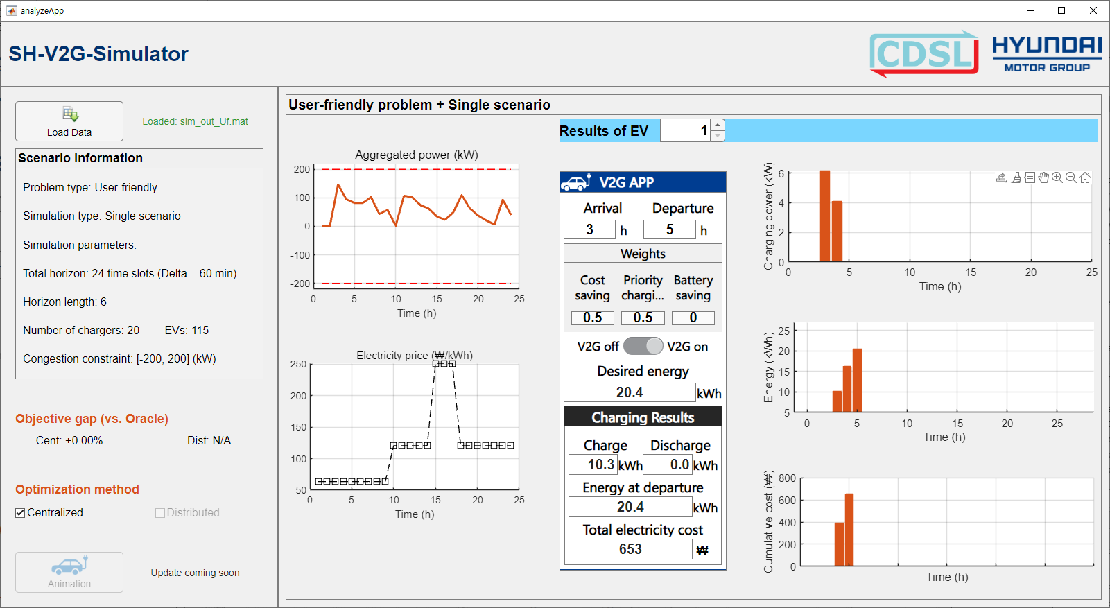
analyze helps evaluate the user-level performance, especially in terms of each user’s preference fulfillment.

Analyze Monte-Carlo Result (Load Flattening)

In this example, the output of simulate_mc() function for a load flattening scenario is required. It can be generated manually following the earlier example, or obtained from the mc_out_Lf.mat located in the tutorial/Samples/ folder.

% Load output
mc_out = load("mc_out_Lf.mat");

% analyze()
analyze(data=mc_out);

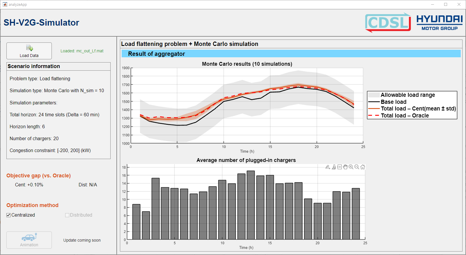
analyze helps examine the average effects across multiple scenarios.

Analyze Monte-Carlo Result (User-Friendly)

In this example, the output of simulate_mc() function for a load flattening scenario is required. It can be generated manually following the earlier example, or obtained from the mc_out_Lf.mat located in the tutorial/Samples/ folder.

% Load output
mc_out = load("mc_out_Uf.mat");

% analyze()
analyze(data=mc_out);

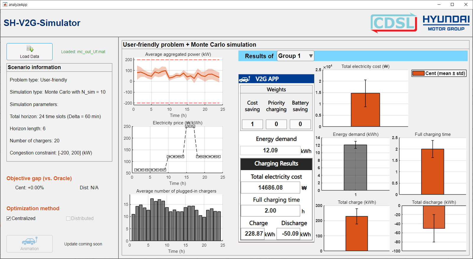
analyze helps examine the average effects across multiple scenarios.